CMO-Aroon Strategy (TMUS)

Momentum Meets Machine: Testing Chande Momentum Oscillator (CMO) and the Aroon indicator

May 01, 2025

Key Performance Metrics Past 5 Years (2020-01-01 until 2025-01-01) TMUS Stock

Trading Strategy Return: 187.10%
Trading Strategy Max Drawdown: 26.04%
Buy and Hold Return: 186.25%
Buy and Hold Max Drawdown: 31.99%
Total Trade: 1 close trade and 1 open trade
Winrate: 100%
Profit Factor: inf
Sharp Ratio: 1.14
CAR: 35.80%
Adjusted CAR (Sharpe-style): 108.68%
Adjusted CAR (Calmar-style): 137.46%
Market Time Exposure: 91.49%

Warning: The returns and results presented are solely based on backtesting using historical data. Although the system has undergone tests to enhance its robustness and resilience to market conditions, there is no guarantee that it will achieve similar profitability in the future. Markets carry inherent risks and volatility. Therefore, you should only invest money that you can afford to lose without causing financial distress.

T-Mobile US Inc. (TMUS) wasn't a stock I initially chose for my portfolio this year, but due to its strong performance, I wanted to develop a trading system that could outperform a simple buy-and-hold strategy. So, I experimented by combining two indicators: the Chande Momentum Oscillator (CMO) and the Aroon indicator. Let's see how the performance turns out.

Overview of the Strategy

The strategy combines 2 momentum indicators:

Chande Momentum Oscillator (CMO): This oscillator measures the difference between gains and losses over a specified period, helping to detect the strength of price movements.
Aroon Indicator: A pair of lines (Aroon Up and Aroon Down) that identify trend changes and the strength of trends based on recent highs and lows.

Walk-Forward Optimization Explained

Walk-forward optimization is a process where a trading strategy is trained on historical data for several years and then tested on the following year to simulate real-world performance. In this case:

The data ranged from 2015 to 2025.
A 4-year training period was used, followed by a 1-year testing period.
Multiple parameter combinations were tested for both indicators, including their periods and signal thresholds.

Each year from 2020 to 2025 was tested with the best parameters found during its prior training period.

Entry and Exit Conditions

Buy signals were generated when:

The CMO was above a certain threshold, and
Aroon Up indicated strong bullish momentum.

Sell signals occurred when:

The CMO fell below a defined level, and
Aroon Down suggested bearish strength.

The signals were backtested with an initial capital of $100,000, taking into account trading fees and slippage to simulate real market conditions.

Full Code Here:

import numpy as np
import pandas as pd
import yfinance as yf
import vectorbt as vbt
import itertools
import matplotlib.pyplot as plt

# CMO Calculation
def calculate_cmo(df, period):
    delta = df['Close'].diff()
    up = delta.clip(lower=0)
    down = -delta.clip(upper=0)
    sum_up = up.rolling(window=period).sum()
    sum_down = down.rolling(window=period).sum()
    cmo = 100 * (sum_up - sum_down) / (sum_up + sum_down)
    return cmo

# Aroon Calculation
def calculate_aroon(df, period):
    aroon_up = 100 * df['High'].rolling(window=period).apply(lambda x: np.argmax(x) / period, raw=True)
    aroon_down = 100 * df['Low'].rolling(window=period).apply(lambda x: np.argmin(x) / period, raw=True)
    return aroon_up, aroon_down

# Walk-forward optimization with CMO + Aroon
def walk_forward_optimization_cmo_aroon(df, start_year, end_year):
    results = []

    # Parameter ranges
    cmo_periods = range(10, 31, 5)
    aroon_periods = range(10, 31, 5)
    cmo_entry_thresholds = range(0, 51, 5)
    cmo_exit_thresholds = range(-50, 1, 5)
    aroon_entry_thresholds = range(30, 81, 10)
    aroon_exit_thresholds = range(30, 81, 10)

    for test_year in range(start_year + 4, end_year + 1):
        train_start = test_year - 4
        train_end = test_year - 1

        train_data = df[(df.index.year >= train_start) & (df.index.year <= train_end)]
        test_data = df[df.index.year == test_year]

        best_params = None
        best_return = -np.inf

        # Try all param combinations
        for params in itertools.product(cmo_periods, aroon_periods, cmo_entry_thresholds, cmo_exit_thresholds, aroon_entry_thresholds, aroon_exit_thresholds):
            cmo_p, aroon_p, cmo_entry, cmo_exit, aroon_entry, aroon_exit = params

            train_data['CMO'] = calculate_cmo(train_data, cmo_p)
            train_data['Aroon_Up'], train_data['Aroon_Down'] = calculate_aroon(train_data, aroon_p)

            entries = (train_data['CMO'] > cmo_entry) & (train_data['Aroon_Up'] > aroon_entry)
            exits = (train_data['CMO'] < cmo_exit) & (train_data['Aroon_Down'] > aroon_exit)

            portfolio = vbt.Portfolio.from_signals(
                close=train_data['Close'],
                entries=entries,
                exits=exits,
                init_cash=100_000,
                fees=0.001,
                slippage=0.002,
                freq='D'
            )

            total_return = portfolio.total_return()
            if total_return > best_return:
                best_return = total_return
                best_params = params

        # Apply best params on test year
        yearly_data = df[(df.index.year >= test_year - 1) & (df.index.year <= test_year)]
        cmo_p, aroon_p, cmo_entry, cmo_exit, aroon_entry, aroon_exit = best_params

        yearly_data['CMO'] = calculate_cmo(yearly_data, cmo_p)
        yearly_data['Aroon_Up'], yearly_data['Aroon_Down'] = calculate_aroon(yearly_data, aroon_p)
        yearly_data = yearly_data[yearly_data.index.year == test_year]

        entries = (yearly_data['CMO'] > cmo_entry) & (yearly_data['Aroon_Up'] > aroon_entry)
        exits = (yearly_data['CMO'] < cmo_exit) & (yearly_data['Aroon_Down'] > aroon_exit)

        portfolio = vbt.Portfolio.from_signals(
            close=yearly_data['Close'],
            entries=entries,
            exits=exits,
            init_cash=100_000,
            fees=0.001,
            slippage=0.002,
            freq='D'
        )

        results.append({
            'Year': test_year,
            'Best_Params': best_params,
            'Test_Return': portfolio.total_return()
        })

    return pd.DataFrame(results)

# Load data
symbol = 'TMUS'
start_date = '2015-01-01'
end_date = '2025-01-01'

df = yf.download(symbol, start=start_date, end=end_date)
df.columns = ['Close', 'High', 'Low', 'Open', 'Volume']

# Run walk-forward optimization
results = walk_forward_optimization_cmo_aroon(df, 2016, 2025)
print(results)

# Apply best signals for each year and combine
combined_entries = pd.Series(False, index=df.index)
combined_exits = pd.Series(False, index=df.index)

for _, row in results.iterrows():
    year = row['Year']
    cmo_p, aroon_p, cmo_entry, cmo_exit, aroon_entry, aroon_exit = row['Best_Params']

    yearly_data = df[(df.index.year >= year - 1) & (df.index.year <= year)]
    yearly_data['CMO'] = calculate_cmo(yearly_data, cmo_p)
    yearly_data['Aroon_Up'], yearly_data['Aroon_Down'] = calculate_aroon(yearly_data, aroon_p)
    yearly_data = yearly_data[yearly_data.index.year == year]

    entries = (yearly_data['CMO'] > cmo_entry) & (yearly_data['Aroon_Up'] > aroon_entry)
    exits = (yearly_data['CMO'] < cmo_exit) & (yearly_data['Aroon_Down'] > aroon_exit)

    combined_entries.loc[entries.index] = entries
    combined_exits.loc[exits.index] = exits

# Filter data for testing period only
df = df[(df.index.year >= 2020) & (df.index.year <= 2025)]
combined_entries = combined_entries[(combined_entries.index.year >= 2020) & (combined_entries.index.year <= 2025)]
combined_exits = combined_exits[(combined_exits.index.year >= 2020) & (combined_exits.index.year <= 2025)]

# Backtest using the combined signals
portfolio = vbt.Portfolio.from_signals(
    close=df['Close'],
    entries=combined_entries,
    exits=combined_exits,
    init_cash=100_000,
    fees=0.001,
    slippage=0.002,
    freq='D'
)

# Parameters
risk_free_rate = 0.02  # Annual risk-free rate, e.g., 2%

# Get core metrics
car = portfolio.annualized_return()
vol = portfolio.annualized_volatility()
max_dd = abs(portfolio.max_drawdown())

# Adjusted CAR using Sharpe-style formula (based on volatility)
adj_car_sharpe = (car - risk_free_rate) / vol if vol != 0 else np.nan

# Adjusted CAR using Calmar-style formula (based on drawdown)
adj_car_calmar = car / max_dd if max_dd != 0 else np.nan

# Initialize variables to track exposure calculation
in_position = False
exposure_days = 0
total_days = len(df)

# Loop through the entries and exits to calculate exposure
for i in range(1, len(df)):
    if combined_entries[i] and not in_position:  # Entry signal (enter position)
        in_position = True
        entry_day = i  # Track entry day
    elif combined_exits[i] and in_position:  # Exit signal (exit position)
        in_position = False
        exit_day = i  # Track exit day
        exposure_days += exit_day - entry_day  # Count days in position

# If the last position is still open (i.e., no exit signal), consider the last day of the dataset
if in_position:
    exposure_days += total_days - entry_day  # Count remaining days in position

# Calculate exposure as percentage of time in position
exposure_percentage = (exposure_days / total_days) * 100

stats = portfolio.stats()
stats['CAR'] = f"{car:.2%}"
stats['Adjusted CAR (Sharpe-style)'] = f"{adj_car_sharpe:.2%}"
stats['Adjusted CAR (Calmar-style)'] = f"{adj_car_calmar:.2%}"
stats['Market Time Exposure'] = f"{exposure_percentage:.2f}%"

# Display performance metrics
print(stats)

# Plot equity curve
portfolio.plot().show()

# Get unique years in the dataset
years = sorted(df.index.year.unique())

# Store annual returns
strategy_returns = {}
buy_and_hold_returns = {}

for year in years:
    yearly_data = df[df.index.year == year]

    if not yearly_data.empty:  # Check if data exists for the year
        # Buy & Hold Return
        start_price = yearly_data.iloc[0]['Close']
        end_price = yearly_data.iloc[-1]['Close']
        buy_and_hold_return = (end_price - start_price) / start_price
        buy_and_hold_returns[year] = buy_and_hold_return

        # Strategy Return
        strategy_returns[year] = results[results['Year'] == year]['Test_Return'].values[0]

# Plot bar chart
plt.figure(figsize=(10, 5))
bar_width = 0.4
plt.bar([y - bar_width/2 for y in strategy_returns.keys()], strategy_returns.values(), width=bar_width, label="Trading Strategy")
plt.bar([y + bar_width/2 for y in buy_and_hold_returns.keys()], buy_and_hold_returns.values(), width=bar_width, label="Buy & Hold")

plt.xlabel("Year")
plt.ylabel("Return")
plt.title("Trading Strategy vs Buy & Hold Annual Returns")
plt.legend()
plt.xticks(list(strategy_returns.keys()))

plt.show()

Result and Analysis

Walk Forward Optimization Result:

Year Best_Params Test_Return
2020 (30, 10, 10, -50, 30, 30) 0.684581
2021 (30, 10, 45, -50, 30, 30) 0.000000
2022 (20, 10, 40, -50, 70, 30) 0.112731
2023 (30, 25, 5, -45, 30, 30) 0.084270
2024 (25, 10, 10, -40, 50, 30) 0.379260
2025 (30, 25, 5, -45, 30, 30) 0.000000

Example:

2025: cmo_p=30, aroon_p=25, cmo_entry=5, cmo_exit=-45, aroon_entry=30, aroon_exit=30

Performance Metrics

Performance Visualization

Buy and Hold Performance Metrics

# Filter Test Years
df = df[(df.index.year >= 2020) & (df.index.year <= 2025)]

# Buy and Hold Performance Metrics
df_holding = df['Close']
pf = vbt.Portfolio.from_holding(df_holding, init_cash=100_000, freq='D')
print(pf.stats())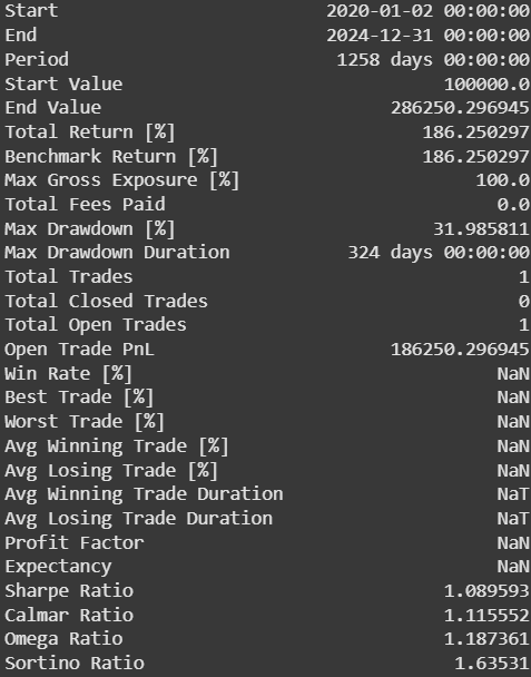

Trading Strategy vs Buy and Hold Annual Return

The backtest results didn’t convince me that this system truly outperforms a buy-and-hold strategy, as the returns were very close. Because of that, I’ve decided to make this trading system freely available. Interestingly, it stays in the market for up to 91% of the time—much higher than most trading systems, which typically remain below 50%.

The one thing this system does relatively well is reducing drawdown. However, even its best strength isn’t all that impressive—it lowers the drawdown from 32% to 26%. Considering it only made two trades in total, I believe there’s still a lot of room for improvement.

Evaluate the Performance of Trading Strategy Relative to a Benchmark

from scipy.stats import linregress

# Calculate Alpha, Beta, and Correlation with a Buy and Hold (B&H) strategy
portfolio_returns = portfolio.returns()
df = df[(df.index.year >= 2020) & (df.index.year <= 2025)]
df_holding = df['Close']
benchmark = vbt.Portfolio.from_holding(df_holding, init_cash=100_000)
benchmark_returns = benchmark.returns()

# Ensure returns are aligned
portfolio_returns, benchmark_returns = portfolio_returns.align(benchmark_returns, join='inner')

# Calculate Beta and alpha using linear regression
slope, intercept, r_value, _, _ = linregress(benchmark_returns, portfolio_returns)
beta = slope
alpha = intercept

# Calculate Correlation
correlation = portfolio_returns.corr(benchmark_returns)

# Display results
print(f"Alpha: {alpha:.4f}")
print(f"Beta: {beta:.4f}")
print(f"Correlation: {correlation:.4f}")

Result

Alpha: 0.0001
Beta: 0.8880
Correlation: 0.9421

Alpha: 0.0001
- It represents the average excess return this strategy generates independent of market movement.
- A value of 0.0001 means this strategy barely outperforms the benchmark after adjusting for market movement—essentially negligible.
Beta: 0.8880
- It measures the sensitivity of this strategy to the benchmark (Buy and Hold).
- A beta of 0.8880 means this strategy tends to move 88.8% as much as the benchmark. It’s less volatile than the benchmark.
Correlation: 0.9421
- This tells you how closely returns move with the benchmark.
- A correlation of 0.9421 is very high—it means this strategy’s returns are strongly in sync with Buy and Hold, even though the trades are different.

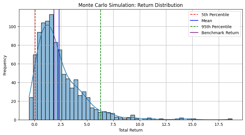
Monte Carlo Simulation

# ------------------ ADVANCED MONTE CARLO SIMULATION ------------------
import seaborn as sns

# Parameters
n_simulations = 1000
n_days = len(portfolio.returns())
init_value = 100

# Get daily returns from the backtest
returns = portfolio.returns().copy().values  # convert to numpy

# Prepare to store metrics
equity_paths = []
drawdowns = []
final_returns = []
sharpe_ratios = []
volatilities = []

# Define Benchmark Return and Max Drawdown
benchmark_return = 1.8625
benchmark_drawdown = 0.3199

# Counters for number of simulations below benchmark return or above benchmark drawdown
below_benchmark_return_count = 0
above_benchmark_drawdown_count = 0

# Simulate full paths
for _ in range(n_simulations):
    sampled_returns = np.random.choice(returns, size=n_days, replace=True)
    equity = init_value * np.cumprod(1 + sampled_returns)

    equity_paths.append(equity)
    daily_returns = np.diff(equity) / equity[:-1]

    max_dd = np.max(1 - equity / np.maximum.accumulate(equity))
    total_return = (equity[-1] / init_value) - 1
    volatility = np.std(daily_returns)
    sharpe = np.mean(daily_returns) / (volatility + 1e-8) * np.sqrt(252)  # Avoid div by zero

    drawdowns.append(max_dd)
    final_returns.append(total_return)
    volatilities.append(volatility)
    sharpe_ratios.append(sharpe)

    # Count simulations below benchmark return and above benchmark drawdown
    if total_return < benchmark_return:
        below_benchmark_return_count += 1
    if max_dd > benchmark_drawdown:
        above_benchmark_drawdown_count += 1

# Plot: Sampled equity paths
plt.figure(figsize=(12, 6))
for i in range(50):  # only plot 50 to avoid clutter
    plt.plot(equity_paths[i], alpha=0.2, linewidth=0.8)
plt.title('Monte Carlo Simulated Equity Curves (50 of 1000)')
plt.xlabel('Days')
plt.ylabel('Portfolio Return')
plt.grid(True)
plt.show()

# Plot: Histogram of final returns with benchmark line
plt.figure(figsize=(10, 5))
sns.histplot(final_returns, bins=50, kde=True)

# Add percentile, mean, and benchmark lines
plt.axvline(np.percentile(final_returns, 5), color='red', linestyle='--', label='5th Percentile')
plt.axvline(np.mean(final_returns), color='blue', linestyle='-', label='Mean')
plt.axvline(np.percentile(final_returns, 95), color='green', linestyle='--', label='95th Percentile')
plt.axvline(benchmark_return, color='purple', linestyle='-', label='Benchmark Return')  # Benchmark Line

plt.title('Monte Carlo Simulation: Return Distribution')
plt.xlabel('Total Return')
plt.ylabel('Frequency')
plt.grid(True)
plt.legend()
plt.show()

# Plot: Histogram of drawdowns with benchmark line
plt.figure(figsize=(10, 5))
sns.histplot(drawdowns, bins=50, kde=True, color='salmon')

# Add percentile, mean, and benchmark lines
plt.axvline(np.percentile(drawdowns, 5), color='red', linestyle='--', label='5th Percentile')
plt.axvline(np.mean(drawdowns), color='blue', linestyle='-', label='Mean')
plt.axvline(np.percentile(drawdowns, 95), color='green', linestyle='--', label='95th Percentile')
plt.axvline(benchmark_drawdown, color='purple', linestyle='-', label='Benchmark Max Drawdown')  # Benchmark Line

plt.title('Monte Carlo Simulation: Max Drawdown Distribution')
plt.xlabel('Max Drawdown')
plt.ylabel('Frequency')
plt.grid(True)
plt.legend()
plt.show()

# Show summary stats
print("Monte Carlo Summary (1000 Simulations):")
print(f"Mean Final Return: {np.mean(final_returns):.2%}")
print(f"Median Final Return: {np.median(final_returns):.2%}")
print(f"5th Percentile Return: {np.percentile(final_returns, 5):.2%}")
print(f"95th Percentile Return: {np.percentile(final_returns, 95):.2%}")
print(f"Average Max Drawdown: {np.mean(drawdowns):.2%}")
print(f"Average Sharpe Ratio: {np.mean(sharpe_ratios):.2f}")

# Print number of simulations below benchmark return and above benchmark max drawdown
print(f"Number of simulations with return less than benchmark: {below_benchmark_return_count}")
print(f"Number of simulations with max drawdown greater than benchmark: {above_benchmark_drawdown_count}")

Monte Carlo Simulate

Return Distribution

Max Drawdown Distribution

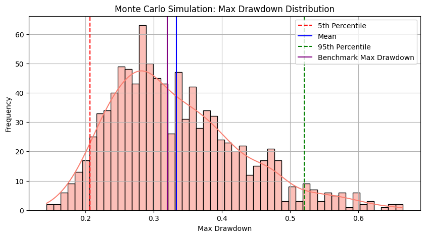
Monte Carlo Summary (1000 Simulations):
Mean Final Return: 234.05%
Median Final Return: 175.00%
5th Percentile Return: 7.14%
95th Percentile Return: 628.66%
Average Max Drawdown: 33.36%
Average Sharpe Ratio: 0.93
Number of simulations with return less than benchmark: 530
Number of simulations with max drawdown greater than benchmark: 481

The result from the Monte Carlo simulation also turned out as expected — it doesn’t provide much of an edge over Buy and Hold. There’s about a 50/50 chance that the trading system will either outperform or underperform Buy and Hold.

Therefore, it might be necessary to avoid over-filtering the signals, perhaps by switching from using two momentum indicators to incorporating a volume-based indicator instead.

Kridtapon P.

Discussion about this post